
How to skip rows in an Excel formula?
There is nothing more frustrating in MS Excel and Google Spreadsheets than their inability to recognize a pattern in referenced cells.
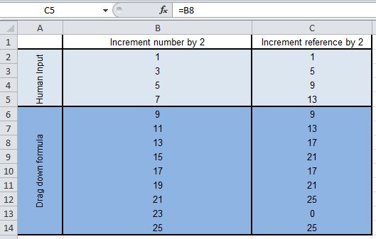
For example, if you type 1, 3, 5 and 7 in four cells and then drag them down, Excel knows that the next in series is 9, 11, and 13 etc.
However, if you type =B2, =B4, =B6 and =B8 in four cells and then drag them down, Excel does not know that the next in line should be =B10, =B12, =B14 and so on.
Even Google Spreadsheet doesn’t do this and I don’t know if this is a feature or a bug but I’m leaning towards a bug, as I’ve felt the need for this many many times, and although there are workarounds to do this I haven’t seen any really easy ways to do it until recently.
After breaking my head on the Offset function for a few hours today I started searching for a new solution to do this and stumbled upon this neat find and replace trick to skip rows while using them in a formula.
What you do is instead of typing =B2, =B4, =B6 and =B8 in four cells and then dragging them down, type something like $B2, $B4, $B6 and then drag it down. Excel will correctly populate the series for you now.
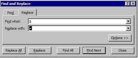
After that all you have to do is select your cells and find and replace the dollar sign with the equal sign to convert the cells into a formula and voila — you have the correctly referenced cells.
This is one of the most useful Excel tricks that I’ve ever come across, and I’m really amazed at the simplicity and the effectiveness of this. Anyone who has tried to do this using round about ways will realize how much time this will save, and how useful this is becase there are just countless times that you need to skip rows while using them in an Excel or a Google Spreadsheet formula.
I haven’t understood the problem correctly. If the series in the coloumn B is to be repeated in col C with an increment of 2, one could enter in cell C2=B2+2 and drag cell C2 down. Then in Col C the numbers will appear as 3, 5, 7 etc.
I must confess that though I have been using Excel extensively since 1982, I am still a novice. For instance, I did not know how to give index for the numerous sheets in a workbook in a contents page so that by clicking the item one can go to the sheet. The procedure is as follows:
1. At a cell in the Contents page Right click and select hyperlink. It would lead to a window.
2 Assuming the title given below the sheet is Population-Bom
In the first cell type #’Population-Bom’!A1
3. In the other cell appearing in the window type how you want that reference to appear say Bombay population 2011 and press OK.
4. Make sure that the name entered in 2 above should be exactly the same with spacing etc. To ensure this one can copy the title from the sheet and paste in step 2.
There is a simpler way of viewing the sheets by pressing ALT+F11
Thank you for your tip, it is very useful.
I’m afraid I didn’t do a good job in explaining the problem. The problem is not that the number has to be incremented by 2. The problem is that the reference cell has to be incremented by 2. So, I need the values of B2, B4, B6 in cells C1, C2, and C3 respectively.
Elegant solution to a nagging problem, thank you.
This just saved me a whole bunch of time!